Random forest analysis example

Random Forest Analysis: A Workflow for Identifying Predictive Variables

Random forest analysis is a powerful machine learning technique used to understand the relationship between predictor variables and response variables. In research, this process typically involves several key steps: data generation, accounting for collinearity, dividing data into training and testing sets, training the model, fine-tuning, and evaluating predictions on test data.

I’ll use examples from a collaborative research project to demonstrate the essential workflow of random forest modeling. The study aimed to identify predictor genes responsible for phenotypic variations. The details of this study have been anonymised and simplified to maintain confidentiality while illustrating the workflow and data interpretation. This approach is widely adopted in biological research, such as for drug discovery or evaluating the efficacy of interventions.

Accounting for Collinearity

First, I tested for collinearity among the predictor variables to remove those that were highly correlated before building the models. Highly correlated variables can reduce both modeling efficiency and interpretability.

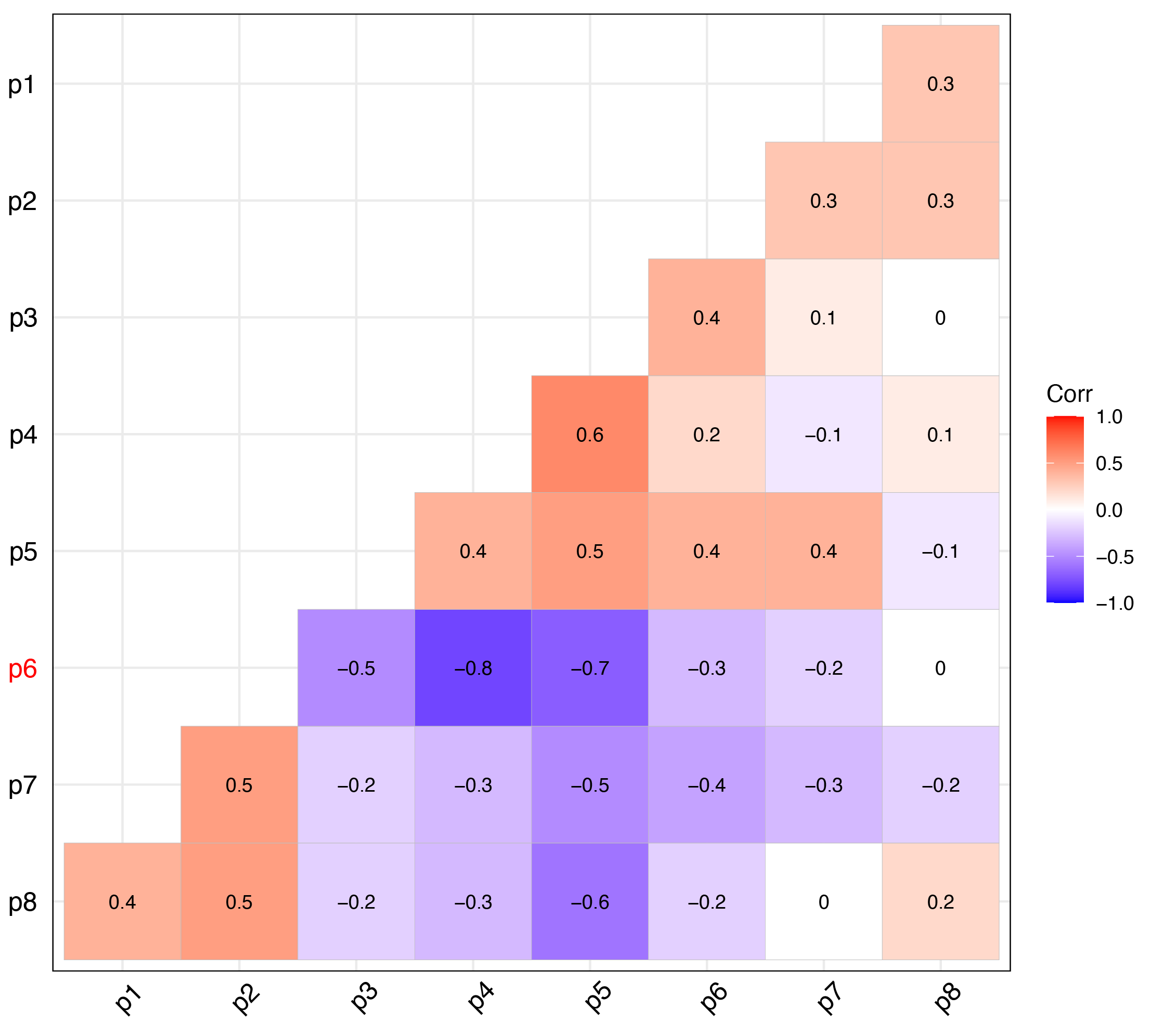
I removed predictor variables with a Pearson correlation coefficient above 0.7 or below -0.7 to ensure the models were not affected by redundancy. In this case, p4 and p6 are highly correlated, and I removed p6.

Dividing the Data

Next, I split the data into a training set (80%) and a testing set (20%). The training set was used to build the random forest models in RStudio.

Fine-Tuning the Model

Based on the model’s performance, I fine-tuned the model to identify the optimal split variables and the ideal number of trees to use. I noticed that the predictions varied slightly with each run due to the randomisation inherent to the random forest method. To address this, I aggregated the predictions using a defined range of seed numbers.

Visualising and Evaluating Predictions

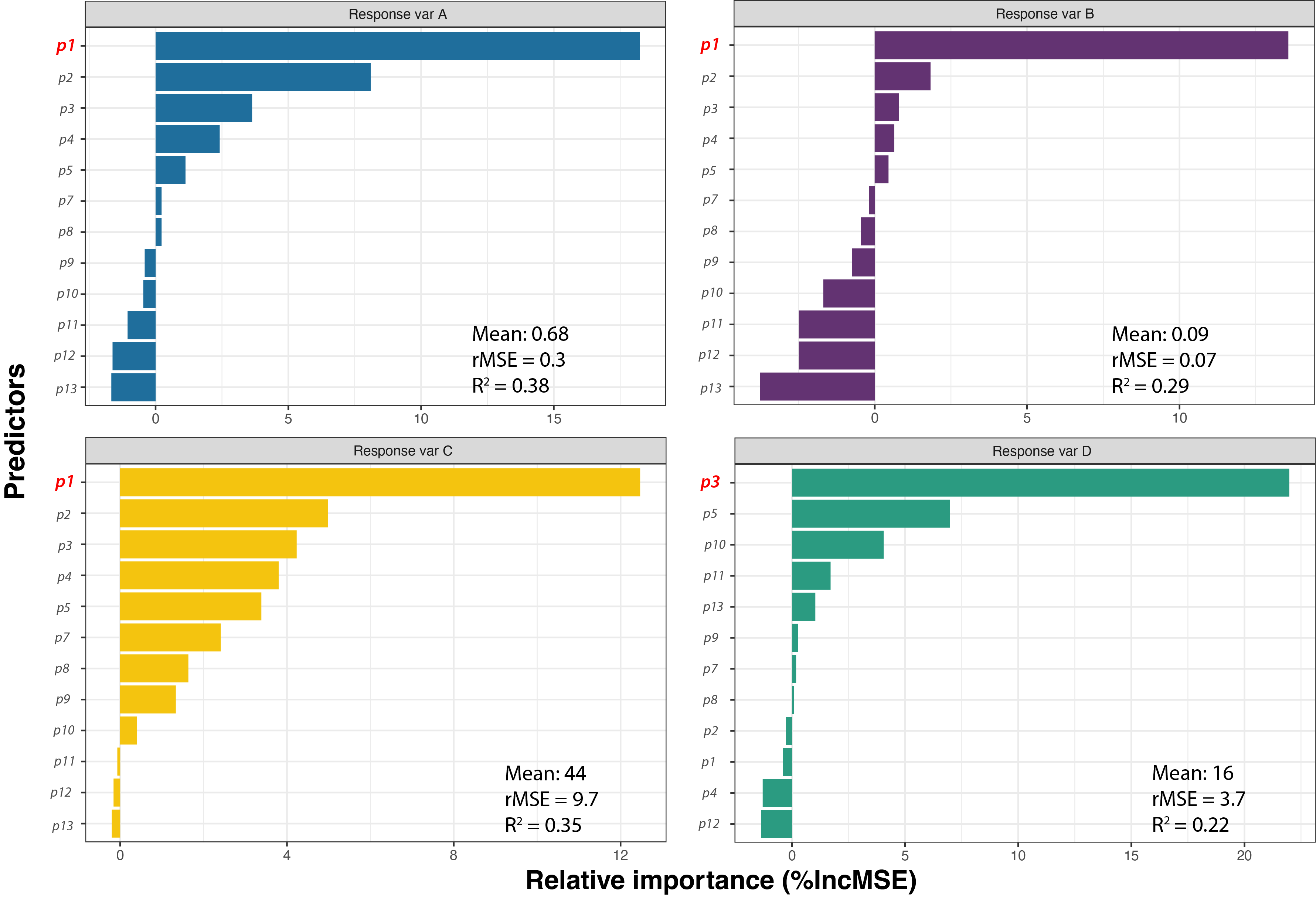
Finally, I visualised the predictions in the following plot to assess model performance and identify the best predictors for each phenotype.

Conclusion

All four models are able to predict between 52% to 78% of the variations in the training dataset, while the error (indicated by rMSE, root of Mean Squared Error) indicates that marginal errors exist between the predictions and actual data. The top predictor is identified by measures the percentage increase in MSE, meaning the increase of modelling error when a certain predictor is removed.

The results showed that p1 was overwhelmingly important for all response variables, except for Response Variable D. This finding helps validate our hypotheses and offers insights into previously unidentified biological mechanisms, i.e. p3.

Implication

This high-level workflow outlines how random forest analysis can be used effectively in biological research. This approach can be easily adapted for use in various research contexts.